Foreword
The goal of the following content is to help you learn applied cryptography. The chapters are in no particular order. Explore!
Introduction to mathematical cryptography
The goal of this section is that you understand some of the first cryptographic protocols. These are the building blocks for more modern cryptography. The contents are incomplete, and we encourage you to search more material if you don't understand something. Let's start with some math.
Math intro
Groups
A group is a fancy mathematical name for a set of elements that are related to each other. These elements are related through an operation called the group operation. This operation must be associative and have a neutral element. The number of elements in the set is called the order of the group.
Example: the integers together with the addition form a group because addition is associative and also they have a neutral element represented by :
Finite groups
A finite group is a group where the set of elements is finite. An example of a finite group is the integers modulo and the operation addition. In modular arithmetic two elements and are equivalent if they have the same remainder modulo . This is noted by .
Example: 4 and 12 are equivalent modulo 8, because they have the same remainder when dividing by 8.
Example: the integers modulo 8, noted by , together with the modular addition form a group: and also they have a neutral element represented by : The sets of elements in the group is .
Multiplicative groups
When choosing as a prime number has an additional property. We define the multiplication as . Where for max *. That is, is the result of multiplying and and taking the remainder of dividing by . If is prime, we also know that for all , there exist an element such that . That is, every element has a multiplicative inverse and we can take as the neutral element. This is due to Fermats little theorem. The only detail is we have to remove the , because it doesn't have a multiplicative inverse. We denote this set without the zero
Example: the integers modulo 7 without the zero, noted by , together with the modular multiplication form a multiplicative group: and also they have a neutral element represented by :
Note that addition and multiplication are associative and commutative. In this case, the groups are called commutative or abelian groups. The only thing that changes between a multiplicative group and additive group is its notation (e.g.: using vs or using / for the neutral element). Mathematically they both have the same properties.
Generators
Let be a group. The span of an element is the set you get by repeatedly applying the group operation over that element. Using multiplicative notation, the span of is . This set is not infinite. Note that a finite group has finite elements, so every element will eventually cycle and for some . If the span of generates all the elements in , we say is a generator of the group. This will happen if the size of the span of is the same as the order of the group. Some elements will generate a subset of all the elements. In this case we will say is a generator of that subgroup.
Example: the following table shows the structure of the multiplicative subgroup .
generator span 1 {1} 2 {1, 2, 4} 3 {1, 2, 3, 4, 5, 6} 4 {1, 2, 4} 5 {1, 2, 3, 4, 5, 6} 6 {1, 6} All the elements in the group generate something. In this case, the spans of 3 and 5 each generate the whole group. The elements 2 and 4 belong to a subgroup where all the properties of a group also hold.
The lagrange theorem states that the order of any subgroup in must divide the order of the whole group.
Example: The multiplicative subgroup associated with has order 6. It's subroups have order 1 (trivial subgroup), 2 and 3. They all divide 6.
Finite field
A finite field is similar to a group but instead of only one operation it defines: addition, substraction, multiplication and division. As natural, substraction is the inverse of addition and the same applies for multiplication and division. As before, the number of elements in the set is called the order of the field. Note that with prime, if we consider all the operations we've seen, can be viewed as a finite field noted as .
Note: has order , and also has a multiplicative group associated with it of order , when considering all non-zero elements. It will be common to refer to this as the group associated with .
Further reading
- An introduction to mathematical cryptography
- Efficient Software-Implementation of Finite Fields with Applications to Cryptography
- To compute the multiplicative inverse efficiently, look into the extended euclidean algorithm.
- To compute the exponentiation efficiently, look at Exponentiation by Squaring.
Diffie Hellman
Motivation
Simmetric cryptography algorithms are used to send secret messages between two parts and . In the literature, and are usually called Alice and Bob. Alice and Bob first agree on a secret key , an encryption function and a decryption function . Then we have the following protocol:
- Alice wants to send to Bob.
- Alice encrypts .
- Alice sends to Bob.
- Bob recovers
A good encryption algorithm must hold the property that no one observing can obtain , even knowing and . That is, cryptographers assume everyone knows the algorithm (but not the secret ). This is known as the Kerckhoffs principle.
Diffie Hellman
How can Alice and Bob agree on a secret securely if they live far away? Diffie-Hellman introduced a solution for this problem in a paper from 1976. Their protocol uses multiplicative groups to agree on a random number securely.
Setup: Alice and Bob agree on a finite group and a generator .
- Alice samples a random and computes .
- Alice sends to Bob.
- Bob samples a random and computes .
- Bob sends to Alice.
- Alice computes
- Bob computes
Note that . So Alice and Bob reached to the same random number .
The security of the algorithm depends on the chosen group . For some groups, computing is easy, but computing is hard. This is called the Discrete Logarithm Problem. Actually, the notation is not used, but you can see where the name comes from. This is why groups are useful in cryptography. You can use the fact that the discrete logarithm problem is hard, to "hide" stuff inside a group.
In step 1, Alice "hides" in the group by computing . Then sending is safe if we assume the attackers cannot solve the discrete logarithm problem. Nowadays, is safe to assume this if we use for a really big . But choosing a secure group is a delicate decision. As hardware and algorithms get better, encryption algorithms have to keep up with it. Other groups such as those found on elliptic curves have become more popular for having a more difficult discrete logarithm problem.
The discrete logarithm problem is an example of a one-way function. That is, a function that is easy to compute but hard to invert.
Elliptic curves
Elliptic curves are defined by two parameters . We say a point belongs to an elliptic curve if:
The good thing about elliptic curves is that you can define an operation and a neutral element noted . The points of the curve and this operation form a group . If you take the addition of points and has a geometric interpretation:
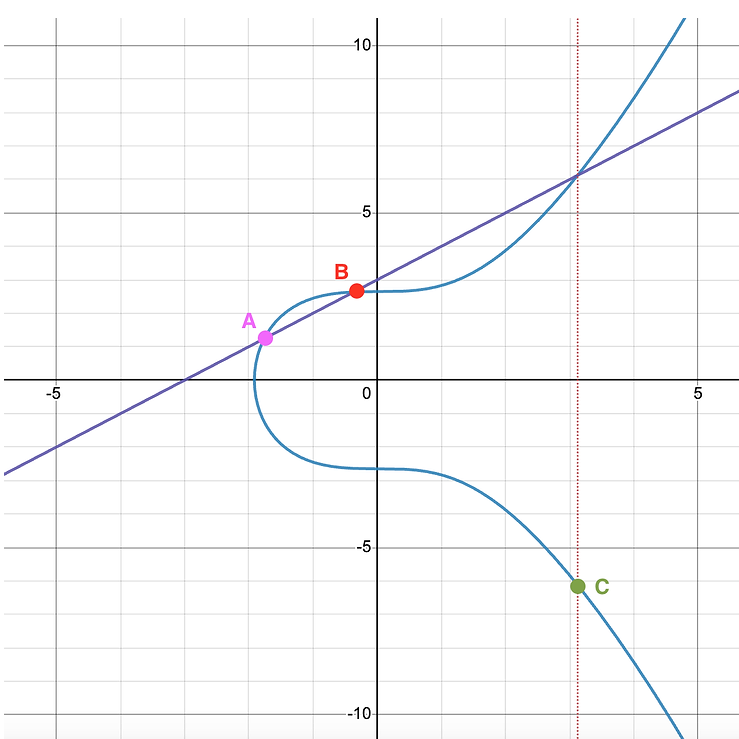
The point is . To add two different points, you find the line that crosses the 2 points. Elliptic curves guarantee that this line will intersect the curve at a third point, then reflect that point over the axis and you get . The inverse of , noted is the reflection we mentioned, the "third point". There are some special cases: when you take a point and its inverse, and when you take the same point twice . This cases form a vertical line that doesn't intersect a third point. Here, we say this line intersects with the point at infinity . This point is the neutral element of .
When adding a point with itself a number of times, we'll use the following notation: .
Curves over finite fields
We are interested in curves where . We'll note the points in the curve . Here, when we plot the points for a specific curve, things get more caotic:
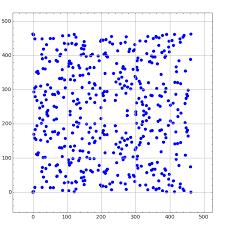
This apparent randomness is what makes elliptic curves useful. For certain combinations of , , and , their group has a difficult discrete logarithm problem. We've seen in the last section why this is useful.
Projective coordinates
When we express the coordinates as , we have to introduce this awkard point that has no actual coordinates. When implementing the curve operation, this leads to bad performance and coding practices. Most implementations of curve operations use projective coordinates instead. This points are represented by such that:
The operations are adjusted accordingly. Each point , has infinite representatives in projective coordinates. If you take the one such that , you're just using affine coordinates. Now we can represent the element as any point .
Families of curves
The curves defined by the equation we've seen so far are said to be in Short weierstrass form. Any elliptic curve can be expressed like this. But there are some more specific families of curves. Some curves can be written in the Montgomery form. Some curves can be written in Edwards form. This curves have additional properties. This properties allow to code faster operations or have more secure groups.
Pairing
The points form a group of order . That is, with different points inside it. A pairing is an operation between two points , that returns an element in :
Do not get confused, we have two different finite fields. is the field where the coordinates of the points live. is the field where things end up after the pairing, this field has the same order as the group of the curve. The pairing has a property called bilinearity:
This property is crazy. It states that adding with itself one more time, is equivalent to multiplying with itself in one more time. It mixes two different worlds. The main algorithm for computing pairings is divided in two steps the Miller loop and the final exponentiation. Most optimizations efforts use properties of specific curves in order to reduce the size of the loop or the exponentiation.
TODO: talk about G1, G2, and field extensions. Maybe do a chapter specific to curves, and keep this more simple.
Introduction to Zero Knowledge Proofs
Disclaimer: this is intended as a first approximation to ZK, most details are not covered and many simplifications have been done for educational purposes.
Introduction
Given a hash function and input , it is easy to obtain . But given , it is hard to find an such that . It is difficult to find the preimage of a hash.
Hashes are used in the context of blockchain to prove you own something. For example, someone can put 100 raccoon-coins in a lockbox and say "Anyone who proves he knows such that , can take this raccoon-coins". Suppose you know . Great! You can claim this juicy coins. But what happens if you want to keep secret to avoid someone else using for future claims?
It would be nice if you could run the following program in your computer:
from hash import H

def claim_raccoon_coins(x):
    # Returns True if user knows the preimage of x.
    y = "0xFF081CAFE"
    return H(x) == y
And generate a proof that convinces anyone that you run the program and it returned True. You wouldn't reveal your secret , because you run the program privately on your computer.
Zero knowledge proving systems consist of a prover and a verifier . First, the prover and the verifier agree on some specific computer program. Then the prover sends to the verifier a proof and a result . This proof convinces that has executed the agreed program and it returned . It is called a zero knowledge proof because it does not reveal any sensitive information. The prover can use secret input parameters and the values of the local variables are not revealed to the verifier. The verifier only knows the instructions and constants, that is, the "text" of the agreed program.
It is desirable that the proof size is small and easy to verify. This property is called succinctness. A common term used in ZK is zkSNARK, this stands for zero knowledge succint argument of knowledge.
General strategy
At first it is hard to imagine how to convince . Specially considering will never see the content of the variables throughout the execution. Let's break down how a ZK proving system works. There are two main components:
- Arithmetization
- Polynomial commitment scheme
Both of these come in different flavours and end up affecting the performance of the system and the proof size. Let's analyze this two components separately and then see how they fit together to make a proof.
Mathematical note: when refering to variables , , they will be elements of a finite field except stated otherwise. This finite field is agreed between and . Understanding finite fields is beyond the scope of this text. Also a domain over this finite field is agreed between the prover and the verifier. This domain is generated by a root of unity .
Arithmetization
The goal of this process is to start thinking about the execution of the program mathematically. We can think of a program as having two important things:
- Memory: a place to store all the intermediate steps of its computation. It can be seen as a vector that stores values.
- Logic: it can be seen as a system of polynomial constraints , that describe which are valid executions.
For a given program, not every "memory" vector will correspond to its logic. Some will be random garbage and some will actually be the intermediate steps of an execution of that program. As programming languages are formal languages, once a program has been written it uniquely defines which corresponds to a valid execution. is just a system of polynomial contraints that is zero when the variables in have the relationship determined by the program:
In zero-knowledge the logic of the agreed program encoded in is known by the prover and the verifier. The content of the computation, encoded in is only known to the prover who has run the computer program. Sometimes is called the witness and is noted by the letter .
This looks confusing at first. Let's see examples of how and look like. There are two different strategies to intuetivily come up with them.
Circuits
The first strategy is to think about the program as a "hardware circuit". This circuit has sum and multiplication gates. Each gate has inputs and outputs. For example, a sum gate has two inputs (x, y) and one output (z). The sum gate enforces the constraint x + y == z. Combining several sum and multiplication gates you end up basically with a complex system of constraints :
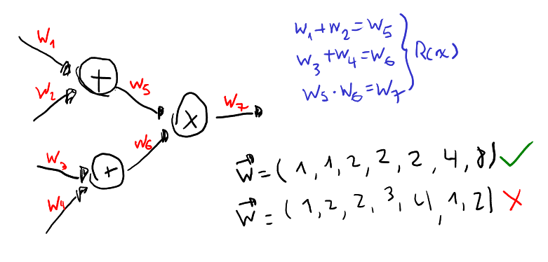
To obtain a witness you can compute the circuit gates. A disadvantage is that circuits are rigid. If you want to prove different programs (other than claim_raccoon_coins), you have to design a different circuit for each of them. Also, using gates is too low-level. There are tools to recycle common circuits called gadgets.
Execution trace
Another strategy is to design a virtual machine. A virtual machine essentially has a set of registers to store values and a set of instructions that describe valid transitions from a state to the following.
Small example
When executing a VM we obtain a series of states. This sequence of states is what we call an execution trace. Here we have the trace of a simple VM that was executed for 3 steps:
OP A B C 1 1 1 2 0 3 2 8 1 3 0 11 This machine is very simple. OP is a register that stores a binary opcode.
AandBstore operands, andCstores the cumulative results (starting at zero). IfOP == 1thenA + Bis added toC. IfOP == 0thenA * Bis added toC. If we see , , and as polynomials such that over the domain , then this can be expressed as the following system of equations :Boundary constraint:
Enforces that the VM starts at zero.
Transition constraint:
Enforces that the next value of
C, represented by , is equal to the sum or product of and , depending on . Remember that this constraints will be evaluated over a domain .Note: and can be obtained through interpolation. In this case the witness is the image of , that is, the result of the computation.
The advantage of this strategy is flexibility. You can code different programs with the VM and they will be accepted. You don't need to design different circuits for different programs. The disadvantage is that you may have performance overhead compared to circuits.
Common practices in constraints
The goal of circuits and execution traces is to intuitively derive the constraints that discriminate correct computation from garbage. If this is not enough for this task, we can add any additional constraints. Here're some frequent practices in proving systems.
Selectors
An example of a selector is the OP column in the execution trace example. Here, a polynomial "selects" which operation is chosen (add or mul). This type of selector polynomials appear frequently inside constraints.
Example:
The selector defines whether or will be equal to .,
Nothing matters
Although this two arithmetization strategies (circuits and execution trace) may seem different, note that both just end up being a system of polynomial constraints . This system is sometimes called R1CS (Rank one constraint system) depending on its form. Having these polynomials in is good, because we need them for our next step: the polynomial commitment scheme.
Polynomial commitment scheme
Polynomial commitment schemes are protocols between the prover and the verifier. In this protocol, commits to a polynomial without revealing any information about to . We say a PCS is binding because the prover can't change the polynomial once he has commited to it (otherwise would notice). A commitment is also hiding because it doesn't reveal unintended information about to .
A normal exchange between and would include three operations called , and . Suppose and want to have an interaction over some polynomial :
[T] := commit(t): the prover computes , the commitment of , and sends it to . From now on, can't change or lie about values without noticing. We'll see why this is useful later. At the moment, you can see as a big number with special properties.proof, t_z := open(t, z): the verifier still doesn't know anything about , but he wants to know for a particular . So the prover computes and aproofto convince .verify(proof, t_z, [T]): using the commitment and the proof, verifies that . The verifier can keep asking the prover to "reveal" the value of at many points, and can't lie about them, can always verify that they come from the same polynomial .
Batch commitments
Usually we want to commit several polynomials, and open them up all at the same point. Most polynomial commitment schemes can be adapted to batch commit and batch open the polynomials, taking advantage of this fact to increase performance.
Example:
[T] := batch_commit(t1, t2, ..., tn)}proof, t1_z, t2_z, ..., tn_z := batch_open(t1, t2, ..., tn, z)batch_verify(proof, t1_z, t2_z, ..., tn_z)
Trusted setup
Some polynomial commitment schemes require a trusted setup. This is a ceremony that generate keys for the prover and the verifier. These keys are needed for the PCS to work. Generally, a trusted third party creates some secret and generates from . Then MUST be thrown away, is called the toxic waste. Having access to the toxic waste would make the protocol insecure.
We have only seen PCS at an abstract level. That's all we need to understand how ZK proofs work. You can later on read about specific schemes suchs as KZG or FRI. Next we'll see how arithmetization and PCSs are used together to generate a ZK proof.
Generating the proof
After arithmetization, both the prover and verifier have a system of polynomial constraints that has the following property:
A good prover knows the correct witness , because it has executed the program. Suppose we encode as a polynomial such that via interpolation. We call this polynomial the witness polynomial. For the zero knowledge property to hold, the prover does not want to reveal the witness to the verifier. The witness could have secret values. The goal of is to convince that he knows such that for all , without revealing . Let's see the whole protocol and then understand how it works.
Protocol
Commitment phase
- computes
- computes such that .
- Commit witness: sends to .
- Commit quotient: sends to .
Challenge and open phase
- sends a challenge to .
- opens and sends the proofs and results to .
Verify phase
- verifies and using the proof following the PCS.
- computes and .
- checks that .
Note: The name of the phases are not common to ZK literature, they where chosen in this text for educational purposes. is sometimes called the quotient polynomial.
Why it works
Commitmment phase
In the commitment phase the prover computes a polynomial called the zerofier. has all the roots we want our polynomial to have. Note that for all if and only if is a valid witness for the program logic encoded in . If is a good prover with a valid witness, then such that can be computed, because divides exactly . After that, the prover commits and and cannot change them anymore. Note that do not reveal any information about the polynomials. These are only commitments.
Challenge phase and open
In the challenge phase, sends a challenge . A challenge it's just a random field element, that cannot know in advance. Note that has committed to and before knowing . cannot have used to craft malicious polynomials during the commitment phase. Now, using the PCS, can send the values and the proof, without revealing any additional information of the polynomial. Special care must be taken, because could choose in order to reveal secret values of . For this purpose, is normally chosen out of the domain .
Verify phase
Note that the verifier could ask for for all using the polynomial commitment scheme. Then, could check that , and infer that is a valid witness, meaning that knows the correct execution of the program! But this has two problems. First, it would not be zero-knowledge, because would reveal the witness to . Second, it would not be succint, because the proof size would be proportional to the witness, which is large. To account for this the Schwartz-Zippel lemma is used. This lemma implies that if you compare two polynomials at a random value and it happens that , then and are the same polynomial with overwhelming probability. This is one of the reasons why we expressed the logic of our computation as a system of polynomial constraints. We want to use this lemma.
First of all, uses the PCS to verify the points and come from the committed polynomials in the first phase, and they have not been changed by a malicious after sending the challenge . Then computes . At this moment, is making sure that the logic of the agreed program is used. also computes the zerofier at , . Next, the verifier checks that . If the prover was good, then this equation must hold. Remember that the constraint system works by discriminating if is a valid witness or garbage. So if divides exactly , then must correspond to a valid witness. The trick for succintness is that we can check that for all , by just checking one equality at holds, by using polynomial division and the Schwartz-Zippel lemma.
Non-interactiveness
The protocol we showed is interactive, in the sense that and talk to each other. We can make this protocol non-interactive if we can get to output the complete proof without asking for a challenge . The challenge step is sometimes replaced with a trick called the Fiat-Shamir heuristic. This is just a way for to sample randomness without asking for it. For this to work, uses the unpredictable output of a hash function over things can't control: the public input, the result of the commitments, etc... The structure used in the algorithms to deliver this randomness is sometimes called the transcript.
Other arguments
There are some common zk-proofs/arguments that are helpful when designing proving systems. You could use these as auxiliary proofs to help your proving system craft the "main proof". Let's see an example.
Permutation argument
The permutation argument is a zk proof on itself. The goal of this argument is to convince that two sets , contain the same elements, without revealing their content. This could be helpful in the context of a bigger proof where you are already using and for some stuff, and you now want to prove the equality of the two sets. As before, the permutation argument will consist of a constraint system.
Out constraint system is inspired in the following fact:
The equation on the right contains polynomials with roots on and respectively. If the sets are equal, then the polynomials are equal, and the reverse is also true. Note that other simpler strategies don't work. For example if we just checked there would be no guarantees about . In this case, there are different ways to obtain the same result : . But polynomials do work, and that is good because as we've already learned, we want to create a system of polynomial constraints in order to make a zk-proof.
Protocol
and agree to work over a finite field and a domain . has polynomials such that and . These polynomials encode and . will prove that , without revealing the contents of the two sets.
Commitment phase
- computes .
- computes .
- sends to .
Commitment phase 2
- sends a challenge to .
- interpolates such that
- computes .
- sends to .
Challenge and open phase
- sends a challenge to .
- opens at .
Verify phase
- verifies .
- verifies that the constraint system holds:
The polynomial constraint system for this particular zk-proof is the following:
We'll interpolate over the polynomial :
This polynomial is the cumulative product of the polynomials we've seen in the last section, until the -th element.
Boundary constraint:
We want the sets to be equal. Once the cumulative product in has reached the end, all the elements are the same and holds. In particular, evaluating that expression in also holds.
Transition constraint:
This constraint makes sure that actually is the cumulative product.
- computes such that
- commits the polynomial and sends it to .
- sends a challenge to .
- opens the polynomial and sends it to .
- verifies using
- verifies
ZK Ecosystem
There are many proving systems. They are very similar between each other. The main differences come from the arithmetization and the PCS used. In this section we'll see different polynomial commitment schemes. If you're not understanding something, go to the "Introduction to ZK Proofs" chapter.
PCS
Next, there is a table with the most popular polynomial commitment schemes. Transparent refers to the trusted setup, FRI doesn't need trusted setup while KZG does.

Minimum data:
- KZG: It is the most succinct of the PCS, but has a trusted setup. Uses elliptic curve cryptography to "hide" data inside the curve group.
- IPA: stands for "Inner product argument", it is a PCS built over another protocol that actually convinces that knows the solution of an inner product. U
- FRI: uses a mix of merkle trees and a low degree test. https://eprint.iacr.org/2022/1216.pdf
Protocols
Some popular protocols are:
- Groth16: first popular protocol. It is from 2016, it has arithmetization based on circuits and uses the KZG polynomial commitment scheme.
- Plonk: similar to groth16, also very popular. Uses circuits and KZG. Its advantage with respect to groth16 is that it encodes the witness more efficiently, and improves performance.
- STARK: can use any arithmetization, but uses the FRI protocol.
KZG
This is a polynomial commitment scheme due to Kate, Zaverucha and Goldberg. It leverages the properties of elliptic curves such as BLS12381. They have two interesting properties. First, the discrete log problem is hard. Second they have a bilinear operation called pairing, that allows for homeomorphic encryption up to one multiplication.
Setup
For KZG to work, an additional step is required at the beginning. This step is called the setup. First, everyone agrees on a group and a generator . Normally is chosen as a high-order prime subgroup of a secure elliptic curve. Then, a trusted third-party samples a random and computes the following:
Then, must be thrown away. Sometimes is called the toxic waste. If someone knew then the PCS would be insecure.
Commit
In the commitment phase wants to commit to a polynomial . To do this, it computes:
Using the homeomorphic properties of the elliptic curve, we can evaluate the encryption of any polynomial at , by just knowing the encryptions of .
Open
The verifier asks for . The prover wants to send , without revealing additional information about (hiding). Also, he wants to convince that he's still using the same polynomial (binding). To do this, computes an auxiliary polynomial . Then, just like in the commitment step it computes:
Then outputs where .
Verify
The verifier accepts if the following is true:
This expression is equivalent to:
Because of the bilinearity, the pairings can be transformed to multiplications in the "plaintext" domain. Also, the multiplications in can be transformed to additions. Then we have that the latter equation holds if and only if the following holds:
This will hold if and only if so the verifier is convinced.
Protocols
This section shows how protocols mix arithmetization techniques and polynomial commitment schemes, to actually obtain provable computation.
Plonk
The plonk paper is well written and the protocol is described in section 8.3. Also, this lambdaclass blogpost is very good. A more concise description is found in section V of this paper.
Hyperplonk
It reduces plonks proof generation time for two reasons:
- Eliminates the need to compute FFTs.
- Better handling of custom gates.
To achieve this, the strategy is to use a ZeroCheck IOP instead of a polynomial quotient. Let's see the different approaches:
- Plonk: uses circuit arithmetization, then interpolates the witness () and selectors (Q_l, Q_r, Q_m, Q_o, Q_c) in univariate polynomials over a domain in .
- Hyperplonk: uses circuit arithmetization, it expresses the witness () and selectors () in multilinear polynomials (with multiple variables of at most degree 1) over a domain , called the Hypercube.

The ZeroCheck requires the prover to do group exponentiations, which is smaller than in Plonk.
Links
- Hyperplonk paper
- Multilinear commitment scheme check out protocol 2
- Plonk paper
Plonky2
Blockchain
At the moment, most of the use cases of zero knowledge technologies are applied in the blockchain industry. Let's see how zk can solve problems in this area.
Ethereum
At its core, Ethereum can be thought of as a global, singleton machine that executes programs given by its users. Unlike traditional centralized systems, Ethereum operates on a blockchain.
Blockchain
A blockchain is a particular type of Peer-to-Peer (P2P) network. These are networks like µTorrent, or the more early ones Ares and Napster. In those cases, the networks store files in a distributed manner without consistency or validity guarantees. In the same way that µTorrent stores files distributed in its nodes to share them, blockchains store another type of data that can be used with other means.
Blockchains store an immutable, but extendable, list (or chain) of messages sent to them. The list gets extended in batches of new incoming messages. Each batch is called a "block" (hench a block-chain). Typically, these messages are called "transactions" because of the more currency-oriented use cases, but in general, a message is just a request sent by a user of the network indicating a desired action. Not every message is valid. Each blockchain has its protocol and accepts incoming messages that conform to certain rules and formats, and that must be consistent with all messages that have already been accepted in previous blocks. Only valid messages are stored in new blocks. Blockchains provide immutability guarantees of the blocks through mechanisms called consensus. Having such an immutable list that can be indefinitely extended with new incoming messages can be used to model different things.
Bitcoin is a blockchain. In this case, the transactions, or messages, that can be stored in the blockchain indicate the movement of funds between addresses of the chain's coin bitcoin. Valid transactions are the ones that request the movement of Bitcoin from accounts that have sufficient funds. That is, from an account for which there exist previous transactions already in the blockchain that moves to them the bitcoins they want to move.
Ethereum
And so, Ethereum is another blockchain. It stores a chain of blocks that ends up modeling a global state machine. Each valid message in this blockchain is either a message that contains the bytecode of a program to store on the blocks, or a request to call a function of an already deployed program. Users and programs get addresses to identify them. And there's a third type of valid message: transferring ether, the Ethereum's coin, from one address to another. And yes, programs can hold ether. At deployment, programs have a hardcoded initial state defined by the developer.
In the same way that in Bitcon's chain, the list of transactions has all the information to recover the balance of every account, in Ethereum the list of blocks of messages is all one needs to recover the global state of the machine. This state, called The World State, is a table with columns "address, balance, program_state". The program state is the state of its variables. This column is empty for every account associated with a regular user that's not a program. The World State table is not stored in any block, but uniquely derived from the list of messages stored in the blockchain.
So in essence that is Ethereum. The consensus mechanism makes sure the blocks are immutable, and the state of the global machine can consistently evolve in time.
Terminology
In the context of Ethereum and blockchain, programs like the ones in the previous section are called "smart contracts", and the messages sent to the blockchain are called "transactions". This is for historical reasons, but it's certainly misleading. That's why we avoided that terminology so far. Since it is so widely used in the field, we will switch to using it from now on.
Token
So what is a Token anyway? A token is a smart contract that maintains a key-value table in one of its variables (therefore in its program state). This key value usually starts with one single entry like {program-owner-address: 10000}, denoting the number of "tokens" held by the owner. And has a send function taking a destination and a value v, and checks whether the sender of the message is in that table and has at least d tokens. Then it will subtract d from its balance and add d to the destination address.
Starknet
At this point you should understand that Ethereum is just a decentralized virtual machine, where anybody can pay money in exchange for running a bit of code. The code is called a smart contract, and when you run or deploy a contract, this is called a transaction. Ethereum has a protocol that guarantees the immutable integrity of all the previous states of this machine, and that guarantees that it evolved correctly.
The problem with ethereum is that transactions are expensive. Each transaction executes a smart contract and the fee you have to pay is proportional to the amount of computation your contract does. If you have a small program you may pay less gas, if you have a large program you pay more gas (Costs reference). The cost of gas depends on the number of transactions that the system has to handle. Unfortunately, this means that when many transactions are in demand, the cost rises too much.
This is sometimes called the blockchain trilemma: you can't have decentralization, security and scalability (low costs) all at the same time. To solve this, L2 layers such as Starknet appeared.
Ethereum is very powerful because it can run turing complete smart contracts. This makes it possible for people to do stuff outside Ethereum, and generate cryptographic proofs that guarantee they sticked to a particular protocol. This cryptographic proofs can then be verified by a contract on Ethereum.
An L2 layer is a blockchain that runs in parallel to Ethereum. Transactions can be executed there instead of Ethereum. Somehow, this transactions are batched. A batch of T transactions in L2 is translated to just only one transaction in the L1, this means that the cost of one transaction can be splitted between T users, reducing the cost. The mechanism has to be good enough, to guarantee the integrity of the L2 blockchain through only one transaction in the L1.
A good strategy to do this is to use zero knowledge. L2 layers using zk to reduce transaction fees in L1, are sometimes called zk rollups.
Starknet architecture
Let's see how starknet can reduce the transaction fees.
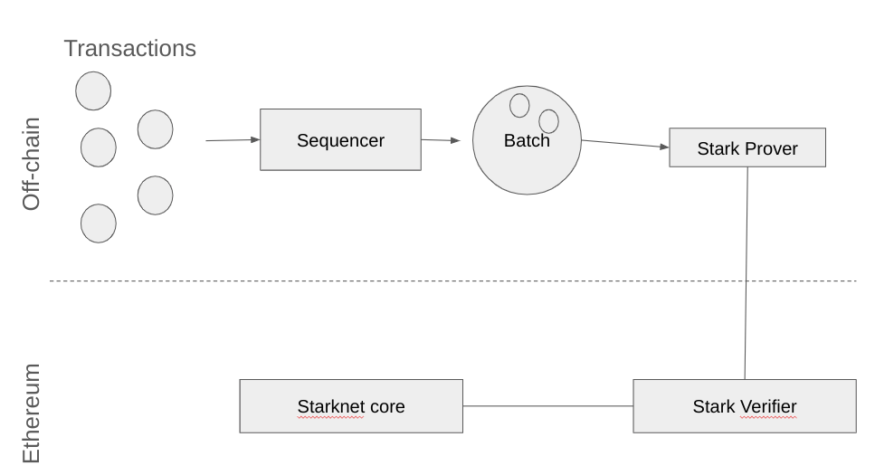
The strategy to do so is the following:
- Alice wants to reduce the fees she's paying for ethereum transactions.
- Alice freezes 100 eth in a smart contract living in the L1 belonging to Starknet.
- Alice can make transactions with other people who have also frozen their eth in Starknet.
- Starknet uses a server (off-chain) to batch this transactions and create a block .
- Starknet uses zero knowledge to prove that applying the transactions in moves the starknet state from to . This is done also off chain.
- A smart contract living in Ethereum, owned by starknet, verifies that the zk-proof is correct.
The verifier in step 6 is sometimes referred as zl roll-up contract.
The state of starknet is encoded in the root of a merkle tree. When transactions are applied, the merkle tree is modified and the new root is computed. The zk-program generates a proof that all this process was done correctly. This roots are called state commitments and are public parameters of the zk-program. This commitments are stored in the L1, guaranteeing the integrity of the L2. At step 6 we have cryptographic certainty that all the transactions where executed correctly and that starknet is not doing anything nasty. People can see the transactions that where executed in L2's in the L1. There's an unexpensive way to do this through calldata, that is, sending data as the input parameter of a dumb smart contract.
The contracts in Starknet are written in a language called Cairo. The specifications of this language have been translated to a system of polynomial constraints, also called AIR (Arithmetic intermediate representation). This constraints can be used to apply a polynomial commitment scheme to produce zk-proofs. The PCS used in starknet is called FRI, and the prover is called Stark prover, because it follows the Stark protocol. This protocol was inventend in part by Eli Ben Sasson, the co-founder and CEO of Starknet.
The transactions are executed twice*. The first time to check that it is a well-formed program, in the sense that it complies with the starknet protocol and it doesn't throw a runtime exception. After this first execution, an execution trace is generated, then a proof can be made out of this.
Further reading
Aztec
Different blockchains provide different functionality. Bitcoin offered decentralized transactions and a currency. Ethereum added turing complete smart contracts, basically a decentralized VM. Aztec aims to build a layer of privacy on top of Ethereum. Other projects such as Z-cash have done this before, but the goal of Aztec is to make private smart contracts, and not just money exchange like Z-cash.
| Technology | Programmable | Private |
|---|---|---|
| Bitcoin | No | No |
| Ethereum | Yes | No |
| Zcash | No | Yes |
| Aztec | Yes | Yes |
Similarly to Starknet, Aztec is an L2 layer developed on top of Ethereum. This means its architecture is composed of two parts:
- On chain contracts: smart contracts deployed to Ethereum that are in charge of guaranteeing the Aztec system is changing from state to state according to a published protocol. This contracts can be programmed in languages like Solidity, that are compatible with the Ethereum instruction set.
- Off chain contracts: smart contracts running outside Ethereum, inside the Aztec ecosystem. This contracts can be programmed using Noir, a language that compiles to zk circuits, where you can use private input.
The contracts in the L1 and L2 interact with each other to provide a number of benefits. The two main benefits are: privacy and reduced cost*. To achieve privacy, the smart contracts living in the L2, written in Noir, can handle private inputs. A prover runs locally on the machine of each user, and generates a proof that he did not mess up with the protocol. We'll see later how you can do this. To achieve reduced costs, a strategy similar to that of Starknet is used. Basically, a sequencer batches transactions and a single validify proof is crafted, to show to a verifier in the L1 that all the transactions in the batch where correctly reflected in the state of the Aztec system. The cost of running the verifier is splitted between all the users that made a transaction, reducing the transaction fees.
The prover in Aztec uses a protocol called Plonk, a protocol that the company has developed. Its arithmetization is through circuits and uses KZG as a polynomial commitment scheme. The first known open-source implementation due to Aztec is Barretenberg, which is written in C++. There are plans to build a prover in Rust (Barrustenberg), and also to change the protocol a little bit (Honk prover).
Further reading
Bitcoin's lack of anonymity
Bitcoin was not designed to allow anonymous transactions. What Bitcoin has is pseudonymity in the form of addresses. Users of Bitcoin found clever ways to obfuscate the history of transactions to make it hard for anyone to trace funds. One strategy used by Bitcoin clients is to generate new addresses instead of reusing always the same one. Another strategy is the use of laundries. These are entities that for a fee would mix different users' funds to hinder traceability. This is practiced despite the clear risk of not getting the funds back. All this motivated the research to come up with a privacy layer over Bitcoin. The first such solution is Zcash.
Zcash
Zcash is a layer 1 blockchain running a fork of Bitcoin. It supports transactions, like in Bitcoin, but where the sender, the receiver, and the amount are encrypted before being broadcasted. It uses ZK proofs to ensure consistency of the entire ledger.
Zerocoin
The development of Zcash has its origins in 2013 in the paper "Zerocoin: Anonymous Distributed E-Cash from Bitcoin". In that paper, the authors proposed the first scheme providing user anonymity. There were previous works in that direction, however, Zerocoin was the first one to achieve anonymity without relying on trusted parties. This was previous to all the modern proving systems for arbitrary computations. Therefore, Zerocoin achieves anonymity through the use of zero-knowledge proofs of knowledge designed for particular problems similar to Schnorr's protocol.
The idea behind Zerocoin was the following. Every user can execute a transaction that would put some bitcoin into a pool of anonymous coins, called zerocoins. Later on, the user can spend from this pool without revealing their identity, or the exact anonymous coin it is using. The magic of zero-knowledge proofs and the clever protocol handles the consistency of the system.
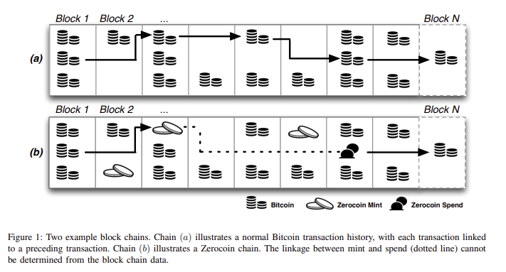
Zerocash
Zerocoin had several problems. The main one was proof sizes. These were in the order of 45kb, making anonymous transactions too large with slow verification times (450 ms). Another problem is that Zerocoin only supports zerocoins of a fixed amount and does not provide means to divide them.
So, in 2014 the paper "Zerocash: Decentralized Anonymous Payments from Bitcoin" was published. It introduces the second generation of these ideas. This time, the proposed protocol achieves privacy and not only anonymity. This means it hides account balances, transaction amounts, and user identities from public view. While doing so, it also improved on every other aspect of Zerocoin: proof sizes were reduced to 1kb, verification times of around 6 ms, anonymous transactions allowed variable amounts, and direct anonymous payments to a user's address. Zerocash leverages one of the first zk-SNARKS for arbitrary programs called Pinocchio.
Zcash
Zcash is the blockchain that implements the Zerocash protocol. Throughout the subsequent years, Zcash evolved following the advances in Zero Knowledge protocols. Different versions of Zcash receive different codenames: Sapling, Sprout, and Orchard. The proving systems used were: BCTV14 in Sapling, Groth16 in Sprout, and Halo2 in Orchard.
References
- Zerocoin.
- Zerocash.
- Pinocchio.
- Zcash 2023 protocol.
- BCTV14.
- Groth16.
- Halo and Halo2.
- CVE-2019-716.
Optimizations
We can fill this chapter with references and brief explanations of how to implement efficient algorithms. It may be operations in curves (addition, pairing) or finite fields (including exp and inv, montgomery form), or other stuff, depending on the needs.
MSM
Pippenger
This is the basic algorithm to optimize MSM. It doesn't leverage curve structure or anything.
- Explained here: Pippenger Algorithm Explained
- Explained also in section 4 here.
GLV Decomposition
- Original paper: Faster Point Multiplication on Elliptic Curves with Efficient Endomorphisms
- To read about endomorphisms: "Guide to Elliptic Curve Cryptography" Darrel Hankerson, Alfred Menezes, Scott Vanstone
- Link it seems that GLV stops being useful after 2^12 points.
Gnark ZPrize optimizations
The original paper is "EdMSM: Multi-Scalar-Multiplication for SNARKs and Faster Montgomery multiplication". This paper explains Pippenger at section 4.
Curve forms and coordinate system
- Mixed addition is adding a point in affine to a point in other coordinate system.
- In a short weierstrass curve, you have different types of coordinate system: affine, projective, jacobian and extended jacobian.
- Uses jacobian extended coordinates. These are the fastest when a curve is in short weierstrass form.
- Uses twisted edwards for mixed addition over BLS* curves.
- Twisted edwards for mixed addition is even better than extended jacobian in short weierstrass. It also uses an extended coordinate system over twisted edwards.
Signed digit decomposition
- When splitting each coefficient of bits into chunks of bits, you end up with possibilities for each coefficient. You can reduce this to using "signed digit decomposition". When a chunk is lower than it stays the same. When a chunk is greater than , then you can substract from it an add to the next chunk .
Parallelization
- Parallelization for pippenger in the "submsms", the first step.
Resources
- Constantine: Nim repo
- Trello card
Security
This is a place where security issues should be explained. Example:
- Discrete Log attacks: Baby-step giant-step for groups of prime order, Pohlig-Hellman for groups whose order is a smooth integer, SSSA attack for curves whose group order is the same as the field order, MOV attack to reduce discrete log in elliptic curves to discrte log in by using pairings, Singular curve reduce a curve to a simpler curve and solve there the discrete log problem.
- Frozen heart (Strong Fiat Shamir)
Links:
Implementing DSA and ECDSA in Crystal
Github repository: https://github.com/ajgara/crystal-primitives
Introduction
Let's explore how we implemented the Digital Signature Algorithm (DSA) in Crystal. The code is available here This includes the implementation of finite fields with their operations and the specific steps to sign a message using DSA.
Crystal is a high-level programming language. It is precompiled and has a garbage collector. Its speed is comparable to Rust and C.
DSA, Digital Signature Algorithm, is an algorithm used for digitally signing a file and authenticating its owner. It is the algorithm that Bitcoin uses to allow wallet owners to authorize transactions.
ECDSA, Elliptic Curve Digital Signature Algorithm, is an advanced digital signature algorithm that uses the principles of elliptic curve cryptography. It is known for its enhanced security and efficiency in comparison to traditional digital signature algorithms like DSA. ECDSA is widely used in various security protocols and systems, including SSL/TLS for secure web communications and in many cryptocurrencies. This algorithm allows for shorter key lengths while maintaining high security, making it a popular choice for modern cryptographic applications.
Crystal does not have developed libraries for cryptographic primitives, so this small work is a first approach in that direction.
Finite Fields in Crystal
To start, we will tackle the implementation of finite fields in Crystal, including their basic operations. This lays the necessary foundation for the development of the DSA algorithm.
Implementing finite fields means creating a Finite Field Element object and implementing field operations on it.
The operations worth mentioning are:
Calculating the Inverse of an Element
This is done using the extended Euclidean algorithm. If is a finite field of order , , then, using the extended Euclidean algorithm, we can find and such that
Since , is the inverse of in .
Calculating the Square Root
The method for calculating the square root of an element in depends on the prime . If , the square root of an element is . Otherwise, the Tonelli-Shanks algorithm must be used.
Implementation
The first important decision to make is where to store the prime that determines the order of the field. The approach suggested in the book "Programming Bitcoin" is to specify the prime every time you create a FiniteFieldElement. In Sagemath, you first create the Field by assigning the prime and then use it to create your elements. Here, we opt for the simplest approach of all, which is to hardcode the prime into the field. We will use . It just so happens that , so it is easy to calculate square roots in .
We use BigInt to store the class representatives of the field. We implement all operations modulo .
Summary of the DSA Algorithm
We will provide a brief summary of the DSA algorithm, highlighting its key components and how they interact to provide secure digital signatures.
DSA is an algorithm for the owner of a private key to sign a message (actually the hash of a message) in such a way that another person can verify the signature using only the signer's public key.
There are some parameters that are public:
- The prime
- A prime such that for some
- A randomly chosen value , usually
The signer has a private key whose public key is To sign the hash of a message , the signer:
-
Chooses randomly and calculates .
-
If , start again with another .
-
Calculate
-
The signature is the pair
The verifier receives the signature and verifies it in the following way:
- Calculates .
- Calculates .
- Calculates .
- Calculates .
- The signature is valid if .
I recommend doing the calculations on paper.
If someone wanted to forge the signature, that is, give a signature for the public key without knowing , then they would need to find a value such that is a solution of , which is essentially solving the discrete logarithm.
Challenges of Implementing DSA in Crystal
We implemented a publicValues class where we store the public parameters: , , , , .
We modeled the signer in a Signer class, which upon initialization generates a private key and derives the public key that can be requested via a method. It has a sign method that signs the hash of a message and returns the signature .
We did not model the Verifier; instead, we implemented a function that takes the message and the signature and performs the calculations to verify it, returning True or False.
The main challenge is a consequence of the decisions we made regarding the prime when implementing finite fields. We had hardcoded the prime as a variable of the class. However, when we want to implement DSA, we are going to make calculations modulo .
Attention to technical details is crucial. It's important to know when you're operating in , when you're in , and when you're in .
I chose to take a shortcut to get everything up and running more or less quickly. We work in when we are in , then if I need to do the calculations modulo , I switch everything to Int and do the calculations modulo . It worked.
Elliptic Curves
We modeled EllipticCurvePoint. Many of the decisions that need to be made when modeling the finite field reappear.
We hardcoded the curve parameters and in the point class. If later we want to generalize to any curve, we will see.
We can create a point on the curve from a pair of BigInt, and the method to create the point verifies if the point is on the curve.
I also implemented a class method to create a curve point from only an , to work more comfortably.
For the neutral element, we added an is_infinity attribute that can be True or False and a class method to create the infinity point.
We implemented equality, addition, and also scalar multiplication.
There is a detail about scalar multiplication. I was tempted to multiply by elements of the field but you can multiply by any integer.
Challenges of Implementing ECDSA
As before, I implemented an ECDSAPublicValues class that holds the public values involved in the signature, which are the generator of the subgroup of the curve, and its order . I also found it convenient to add the prime of the finite field, understanding that it is repeated.
I implemented an ECDSASigner class for signing and a separate function for verification.
When creating a signer, I have to pass a random number generator rng that it uses to create a private key , and then a public key .
To sign a message , I need its hash . Then I randomly draw an element from , obtain , and keep , the first coordinate of , looking at it in . I calculate in and return the signature .
The verifier takes the signature and calculates and . The signature is valid if the first coordinate of is equal to . The difficulty I had was that everything has to be calculated in and not in , since the periodicity of the subgroup generated by and of the field are different.
Next Steps
There were many untidiness in the code. Many times I used integers modulo instead of creating elements of a finite field . This could be quite tidied up. One issue is that the cryptographic protocols themselves do not clarify much where each element lives in each step. Sometimes they start in , then you think of it as an integer, then in . Sometimes they do not even clarify the existence of , only thinking of it as integers modulo .
This is something we could think about and ground.
There is also the option to continue with the book "Programming Bitcoin". And also refactor everything to be able to do calculations with more generic fields and curves.
STARKs sobre BoboVM
BoboVM
Es una máquina virtual simple para construir un protocolo de STARKs con fines pedagógicos.
Estructura general
La máquina tiene 2 registros (, ), una memoria y un conjunto de 4 instrucciones. A medida que se ejecutan una serie de instrucciones el estado de la memoria y de los registros va evolucionando.
Registros
- : el program counter indica qué instrucción se está leyendo.
- : el allocation pointer indica el primer lugar de memoria que todavía no fue escrito.
Memoria
La memoria tiene 256 direcciones que se van escribiendo de menor a mayor. En cada dirección entra algo de 64 bits.
Instrucciones
Hay 4 instrucciones: put, add, jmp y end.
- put [literal_0] : Escribe un literal en la memoria.
- add [literal_0], [literal_1] : suma dos cosas y lo guarda en la memoria.
- jmp [literal_0], [literal_1] : es un salto condicional.
- end : termina el programa.
Codificación
Cada instrucción ocupa 3 bytes repartidos de la siguiente manera:

- dirección_op0 : Una dirección de memoria entre 0 y 255.
- dirección_op1 : Una dirección de memoria entre 0 y 255.
- literal : Guarda un entero entre 0 y 255.
- flags : indica con un 0 o un 1 en el lugar correspondiente qué tipo de instrucción es, solo uno de los flags puede estar encendido al mismo tiempo. Los 8 bits de flags se reparten así:

Los enteros pueden ser positivos o negativos, la interpretación es:
Es decir que guardar un 128 es guardar un 0, guardar un 127 es un .
| inst | code |
|---|---|
| put 3 | 0x00008340 |
| put -1 | 0x00007f40 |
| add [-1], [-2] | 0x7f7e0010 |
| jmp [-1], 1 | 0x7f008104 |
| end | 0x00000001 |
Especificación
-
put [literal] :
- La memoria en pasa a ser [literal]
- Aumenta en 1
- Aumenta en 1
-
add [direccion_op0], [direccion_op1]
- Busca el número de la memoria en la posición + [direccion_op0]
- Busca el número de la memoria en la posición + [direccion_op1]
- La memoria en pasa a ser +
- Aumenta en 1
- Aumenta en 1
-
jmp [direccion_op0], [literal] :
- Busca el número de la memoria en la posición + [direccion_op0]
- Si es cero:
- Aumeta en 1
- Si es distinto de 0:
- pasa a ser [literal]
-
end :
Traza de ejemplo
Llamamos traza a una tabla que guarda los estados sucesivos del programa. El siguiente ejemplo pone un 3 y un -1 en la memoria, después los suma y pone un 2 en la memoria, y luego hace un jump condicional. Como 2 es distinto de cero, vuelve hasta el put -1 y sigue iterando hasta llegar a cero.
put 3
put -1
add [-1], [-2]
jmp [-1], 1
end
Si pudieramos ver la evolución del programa sería algo así (técnicamente la columna instrucción no es parte de esta traza, porque se puede deducir de la memoria y del , la columna clock tampoco porque siempre son los números naturales hasta la cantidad de pasos): | clock | pc | instrucción | ap | | -------- |--------|-------------------|------| | 1 | 0 | put 3 | 5 | | 2 | 1 | put -1 | 6 | | 3 | 2 | add [-1], [-2] | 7 | | 4 | 3 | jmp [-1], 1 | 8 | | 5 | 1 | put -1 | 8 | | 6 | 2 | add [-1], [-2] | 9 | | 7 | 3 | jmp [-1], 1 | 10 | | 8 | 1 | put -1 | 10 | | 9 | 2 | add [-1], [-2] | 11 | | 10 | 3 | jmp [-1], 1 | 12 |
La memoria termina siendo:
| dirección | valor |
|---|---|
| 0 | put 3 |
| 1 | put -1 |
| 2 | add [-1], [-2] |
| 3 | jmp [-1], 1 |
| 4 | end |
| 5 | 3 |
| 6 | -1 |
| 7 | 2 |
| 8 | -1 |
| 9 | 1 |
| 10 | -1 |
| 11 | 0 |
Traza "aumentada"
Dentro de poco vamos a querer expresar restricciones matemáticas sobre la "traza" del programa (la ejecución del mismo). Para expresar estas restricciones de una manera más fácilmente vamos a agregar columnas auxiliares.
La longitud de la traza es exactamente la cantidad de pasos que hizo la máquina durante su ejecución. Vamos nombrando las columnas por secciones:
Columnas de operaciones
| pc | inst | is_add | is_jmp | is_put | is_end | lit |
|---|---|---|---|---|---|---|
| 0 | 0x00008340 | 0 | 0 | 1 | 0 | 3 |
| 1 | 0x00007f40 | 0 | 0 | 1 | 0 | -1 |
| 2 | 0x7f7e0010 | 1 | 0 | 0 | 0 | 0 |
| 3 | 0x7f008104 | 0 | 1 | 0 | 0 | 1 |
| 1 | 0x00007f40 | 0 | 0 | 1 | 0 | -1 |
| 2 | 0x7f7e0010 | 1 | 0 | 0 | 0 | 0 |
| 3 | 0x7f008104 | 0 | 1 | 0 | 0 | 1 |
| 1 | 0x00007f40 | 0 | 0 | 1 | 0 | -1 |
| 2 | 0x7f7e0010 | 1 | 0 | 0 | 0 | 0 |
| 3 | 0x7f008104 | 0 | 1 | 0 | 0 | 1 |
| 4 | 0x00000001 | 0 | 0 | 0 | 1 | 0 |
Columnas de memoria
| ap | val_op0 | add_op0 | val_op1 | add_op1 | write | write_addr |
|---|---|---|---|---|---|---|
| 5 | 0 | 0 | 0 | 0 | 3 | 5 |
| 6 | 0 | 0 | 0 | 0 | -1 | 6 |
| 7 | -1 | 7 | 3 | 6 | 2 | 7 |
| 8 | 2 | 8 | 0 | 0 | 0 | 0 |
| 8 | 0 | 0 | 0 | 0 | -1 | 8 |
| 9 | -1 | 9 | 2 | 8 | 1 | 9 |
| 10 | 1 | 10 | 0 | 0 | 0 | 0 |
| 10 | 0 | 0 | 0 | 0 | -1 | 10 |
| 11 | -1 | 11 | 1 | 10 | 0 | 0 |
| 11 | 0 | 12 | 0 | 0 | 0 | 0 |
| 11 | 0 | 0 | 0 | 0 | 0 | 0 |
Restricciones de transición
Desempaquetado de instrucción
$$\text{inst}=\text{add_op0} * 2^{24} + \text{add_op1}*2^{16}+\text{lit}*2^{8} +\text{is_put}*2^{6}+\text{is_add}*2^{4}+\text{is_jmp}*2^{2}+\text{is_end}$$
Indicador de operación
$\text{is_add} (\text{is_add} - 1) = 0$ $\text{is_mul} (\text{is_mul} - 1) = 0$ $\text{is_put} (\text{is_put} - 1) = 0$ $\text{is_end} (\text{is_end} - 1) = 0$ $\text{is_add} + \text{is_mul} + \text{is_put} + \text{is_end} - 1= 0$
Evolución de PC
Casos que no son jmp: $(1 - \text{is_jmp})(pc'-(pc+1))=0$
Caso de jmp que salta: $\text{is_jmp}\text{val_op0}(pc'-\text{lit})=0$
Casos de jmp que no salta: $\text{is_jmp}(1-\text{val_op0}\text{val_op0}^{-1})*(pc'-(pc + 1))=0$
La columna virtual $\text{val_op0}^{-1}$ tiene el inverso de val_op0 y vale 0 cuando val_op0=0.
Evolución de AP
Suma
$\text{write}=\text{val_op0}+\text{val_op1}$ $\text{addr_op0}=ap+\text{lit1}$
Put
$\text{write}=\text{val_op0}$ $\text{write_addr}=ap$
Restricciones de memoria
More resources
Reading material
Introduction
Elliptic curves
Polynomial commitment schemes
Protocols
Other
- Cryptohacks: a fun website to learn math and all type of cryptographics by solving puzzles and CTFs.