Arithmetization

The goal of this process is to start thinking about the execution of the program mathematically. We can think of a program as having two important things:

• Memory: a place to store all the intermediate steps of its computation. It can be seen as a vector $\vec{x}$ that stores values.
• Logic: it can be seen as a system of polynomial constraints $R(\vec{x})$, that describe which $\vec{x}$ are valid executions.

For a given program, not every "memory" vector $\vec{x}$ will correspond to its logic. Some $\vec{x}$ will be random garbage and some $\vec{x}$ will actually be the intermediate steps of an execution of that program. As programming languages are formal languages, once a program has been written it uniquely defines which $\vec{x}$ corresponds to a valid execution. $R(\vec{x})$ is just a system of polynomial contraints that is zero when the variables in $\vec{x}$ have the relationship determined by the program:

$$R(\vec{x})=0⟺\vec{x}\text{ follows the expected logic of the program}$$

In zero-knowledge the logic of the agreed program encoded in $R$ is known by the prover and the verifier. The content of the computation, encoded in $\vec{x}$ is only known to the prover who has run the computer program. Sometimes $\vec{x}$ is called the witness and is noted by the letter $\vec{w}$.

This looks confusing at first. Let's see examples of how $R$ and $\vec{w}$ look like. There are two different strategies to intuetivily come up with them.

Circuits

The first strategy is to think about the program as a "hardware circuit". This circuit has sum and multiplication gates. Each gate has inputs and outputs. For example, a sum gate has two inputs (x, y) and one output (z). The sum gate enforces the constraint x + y == z. Combining several sum and multiplication gates you end up basically with a complex system of constraints $R(\vec{x})$:

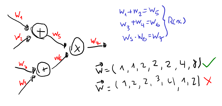
To obtain a witness $\vec{w}$ you can compute the circuit gates. A disadvantage is that circuits are rigid. If you want to prove different programs (other than claim_raccoon_coins), you have to design a different circuit for each of them. Also, using gates is too low-level. There are tools to recycle common circuits called gadgets.

Execution trace

Another strategy is to design a virtual machine. A virtual machine essentially has a set of registers to store values and a set of instructions that describe valid transitions from a state to the following.

Small example

When executing a VM we obtain a series of states. This sequence of states is what we call an execution trace. Here we have the trace of a simple VM that was executed for 3 steps:

OP	A	B	C
1	1	1	2
0	3	2	8
1	3	0	11

This machine is very simple. OP is a register that stores a binary opcode. A and B store operands, and C stores the cumulative results (starting at zero). If OP == 1 then A + B is added to C. If OP == 0 then A * B is added to C. If we see $op$, $a$, $b$ and $c$ as polynomials such that $$op({\omega }^i)=O{P}_i;a({\omega }^i)=A_i;b({\omega }^i)=B_i;c({\omega }^i)=C_i$$ over the domain ${\omega }^i$, then this can be expressed as the following system of equations $R(x)$:

Boundary constraint:

$c({\omega }^0)=0$

Enforces that the VM starts at zero.

Transition constraint:

$c(\omega x)=op(x)\ast (a(x)+b(x)+c(x))+(1-op(x))\ast (a(x)\ast b(x)+c(x))$

Enforces that the next value of C, represented by $c(\omega x)$, is equal to the sum or product of $a(x)$ and $b(x)$, depending on $op(x)$. Remember that this constraints will be evaluated over a domain ${\omega }^i$.

Note: $a,b$ and $c$ can be obtained through interpolation. In this case the witness $\vec{w}$ is the image of $c({\omega }^i)$, that is, the result of the computation.

The advantage of this strategy is flexibility. You can code different programs with the VM and they will be accepted. You don't need to design different circuits for different programs. The disadvantage is that you may have performance overhead compared to circuits.

Common practices in constraints

The goal of circuits and execution traces is to intuitively derive the constraints $R(\vec{x})$ that discriminate correct computation from garbage. If this is not enough for this task, we can add any additional constraints. Here're some frequent practices in proving systems.

Selectors

An example of a selector is the OP column in the execution trace example. Here, a polynomial $op(x)$ "selects" which operation is chosen (add or mul). This type of selector polynomials appear frequently inside constraints.

Example: $$s(x)A+(1-s(x))B=C$$

The selector $s(x)$ defines whether $A$ or $B$ will be equal to $C$.,

Nothing matters

Although this two arithmetization strategies (circuits and execution trace) may seem different, note that both just end up being a system of polynomial constraints $R(\vec{x})$. This system is sometimes called R1CS (Rank one constraint system) depending on its form. Having these polynomials in $R$ is good, because we need them for our next step: the polynomial commitment scheme.